


Laying the groundwork for data-driven evolution
🧬 🔢 Gathering quantitative genotype → fitness data at scale: Part 1


Introduction
Pioneer Labs is engineering microbial evolution to optimize performance on tasks such as biomanufacturing on Mars. But what's the BEST way to achieve this? Natural evolution, fully AI-driven design, or something in between? At Pioneer Labs, we believe in data-driven research. We aim to gather real, quantitative data on the fitness changes that result from evolution and engineering, then measure which approach is best. Furthermore, we need to gather this data at scale in order to enter the regime of big data and unlock the path for computationally driven projects using tools such as machine learning.
With an eye to these long-term goals, we are already establishing experimental platforms that will pave the way for big data efforts. This is the first of two articles that describe our bioinformatics approach, which yields quantitative measurements of evolutionary fitness at scale.
Previously we described our prototype engineering crank, which generates extremophile gDNA libraries and leverages evolutionary selection to find gDNA fragments that convey fitness advantages in high pressure environments such as high salt. Purifying out winners of these selection experiments yields high-fitness strains analogous to natural selection, only faster. With this experimental setup, we are already finding hits!

Can we do even better than just finding the top hits? What if we could quantify the fitness of every gDNA fragment in our library and look for not-quite-top hits? Can knowledge of medium fitness almost-winners help us understand WHY things are conferring fitness advantages? Conversely, can we learn anything from fitness losers? Furthermore, can fitness measurements at scale enable data-driven approaches with tools such as machine learning?
With modern DNA sequencing technologies, we can affordably sequence each individual fragment in our pooled library and measure evolutionary fitnesses in our selection experiment at the single-fragment level. Following the methodology used in the BOBA-seq paper, we use long-read sequencing to associate the full-length fragment (~10kb) with short barcodes, and we infer fitness by reading short-read sequencing to count barcodes at scale over many timepoints.
The punchline: We can measure quantitative genotype → fitness data at the scale of 106-member libraries every time we run an evolution or engineering experiment! This improvement scales up our hit detection rate from highest fitness winners to hits across the entire genome. Scientifically, these datasets extend our ability to detect selection-relevant genes and operons and unlock big data modeling approaches.

Experimental details
We previously used salt tolerance as a Mars-relevant phenotype to prove out reliably quantifying dose-response curves for individual hits. Here, we use salt tolerance again for our proof of concept experiment, replacing the dose-response readout with a high-throughput bioinformatics approach. We generated a large fragment library from the H. elongata genome, a known halophile that thrives in salty conditions. We sequenced the base library with PacBio HiFi sequencing to view the fragments and link them to randomly generated barcodes.
Our full experimental protocol is described in our previous post. Briefly, we transformed E. coli with the fragment library and grew them up overnight in normal LB media. Then we passaged them into 4% salt media for five days, taking a replicate from each day for Illumina sequencing prep
Before looking for scientific insights, we checked our sequencing results’ quality. Below we describe our preliminary characterizations.
Barcoded libraries of extremophile gDNA fragments
We can characterize our libraries in terms of fragment length and genome coverage via PacBio HiFi long-read sequencing.
Our cloning strategy should yield a library with the following properties:
gDNA sequence fragments of ~1-10kb
Even(ish) coverage of the extremophile genome with at least 100x depth
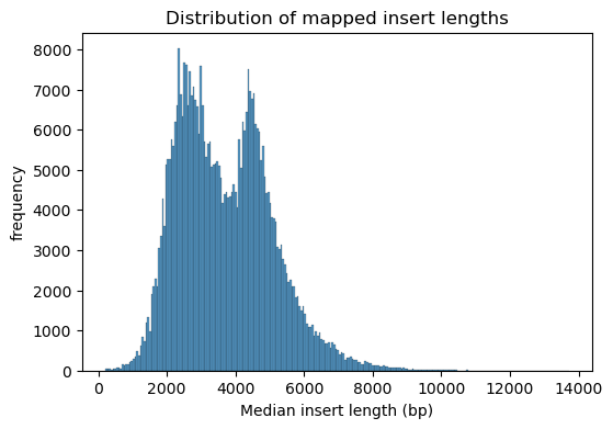
From the PacBio data, we can examine the distribution of mapped fragment lengths. We see that the vast majority of sequences are between 1kb and 8kb. Eventually we’d like to produce larger sequence fragments and wider size ranges – this is a potential area of improvement!
We can define coverage by calculating how many fragments map to each region in the genome. We see that the coverage is relatively evenly distributed, and that the depth typically ranges from 200x to 800x. It’s important to note that this isn’t sequencing depth, but rather genome coverage in our library – each position in the genome is covered by 100-600 unique gDNA fragments, each of which are then sequenced deeply. With coverage this high, we can make quantitative statements about the fitness importance of precise locations in the genome!

Characterizing fragment effects through sequencing selection experiments
We characterize our selection experiments in terms of barcode diversity and frequency trajectories across time via Illumina short read sequencing.
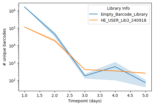
First, we can examine the strength of selection. Over time, we expect barcode diversity to dramatically decrease as low-fitness fragments are out-competed. This is clearly exhibited in the sequencing data – below we show the (log10) number of uniquely sequenced barcodes in both our fragment library as well as a control library possessing just barcodes with no fragments over time in a selection experiment. Both drop to a few hundred species by Day 3, but the fragment library has slightly more (~500 vs ~100) at later timepoints, especially at Day 5, indicating the presence of winners! Interestingly, there is some variability in the control library at Day 4, likely due to some heterogeneity in the cloning strain that confers slight fitness advantages.
Because we sequence every timepoint, we can construct frequency trajectories of individual barcodes over time. From this data we can already detect winners on the basis of increasing frequency over time by looking for trajectories that increase over time and then examining the mapped genes from our PacBio data!
In the below plot we show trajectories of two winning barcodes (with mapped gene content) along with three randomly chosen barcodes. We replicated our earlier hit of opuE. In addition, the clear winner here was galE, a new hit that was not discovered in our earlier experiments. We believe that’s due to fragment size – here our fragments are longer (~5kb) and the functional salt tolerance of galE fragments could require longer sequence fragments than our older library (~1kb) possessed. For both hits, the frequencies increased substantially over time compared to randomly selected barcodes, which quickly died out by Day 2. Losers will decrease over time due to selection pressure, whereas winners increase over time due to evolutionary fitness advantage.

Developing a statistical framework for detecting high-fitness hits at scale
While the biggest winners will be obvious, additional learnings can be gleaned from smaller-effect hits. How do we construct a statistical framework for doing so?
Due to unavoidable cloning inefficiency, many barcodes will lack an inserted fragment sequence – this is expected and even beneficial since they can then be used as an in-sample negative control. By leveraging this negative control, we can calculate a fitness z-score for each barcode. We calculate a log-fold-change in barcode frequency over time (for details, refer to the Boba-seq paper), and then normalize against the empty barcodes to derive a fitness z-score.
Below we show the distribution of fitness z-scores at Day 1 and Day 5 between the empty barcodes and the gDNA fragments. At Day 1 the distributions are virtually identical, whereas by Day 5 the fragment distribution is slightly left-shifted. This indicates that the average gDNA fragment actually imposes a slight fitness burden, e.g. due to wasteful production of nonfunctional RNA.
If we focus on the high fitness values, we see that at Day 5, there are many high-fitness winners present. However, even at Day 1 there are several barcodes that have substantially high fitnesses. The sequencing reveals the presence of subtle higher-fitness hits at early timepoints that we would not have discovered in the previous experimental scheme that relied on late timepoint winners fixing in the population.

Furthermore, because we have this distribution of empty barcodes, we can actually use that as a null distribution for statistical testing and label actual fragment-containing barcodes as statistically significant. For a conservative cutoff, we can use a z-cutoff of 3 (black dashed line), which corresponds to a roughly 0.15% false positive rate. Barcodes that have a higher fitness z-score thus register as significant.
Reproducibility of results
One of the most important aspects of generating large scale data is validating the technical reliability of said data. Below we highlight some control analyses to verify that the numbers we’re generating are indeed quantitatively reproducible.
✅ Technical replicates correlate
Examining barcode-level fitnesses between technical replicates validates the technical success of our bioinformatics-based fitness quantification.
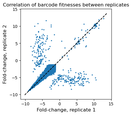
Our experiment contained three technical replicates, and we expect a high degree of correlation in fitness values between replicates. First, we can examine how the fitnesses correlate per barcode. Shown below is an example replicate-replicate scatterplot at Day 3, where each dot is a single barcode. We see that the vast majority of barcodes are neutral-low fitness, but there are a few winners. The ones on the diagonal are reproducibly winning between replicates, whereas the “flanks” are barcodes that win in one replicate but not the other. This is possibly due to effects like clonal interference– the ultimate winners in any single replicate are somewhat random and when they start to dominate the pool, other potential winners may actually die out.
✅ Correlation is even stronger when you view the data ‘per gene’
One major advantage of having long read sequencing data is that now we can map the fragment sequences of each barcode to the reference genome. Thus, each individual barcode can be thought of as an “experiment” on a portion of the source extremophile genome, and multiple fragments covering the same region can provide independent measurements of the same underlying biological phenomenon. This poses the following question: does examining fitness effects at the “genomic region” level provide cleaner numbers than at the single barcode level?
To carry out this analysis, we take each annotated gene body in the reference H. elongata genome and assign it the average fitness of all barcodes that contain that gene body in the fragment sequence.
Collapsing barcodes onto genes improves the correlation between technical replicates and indicates that our selection experiments yield fitness data that are biologically grounded. Below is the same replicate-replicate scatter plot, except now each point is a gene, rather than a barcode. We see that the correlations are quite high, and the “flanks” have disappeared. Essentially, the stochasticity at the single barcode level is no longer present once we average out fitness effects and examine things at the genome level.
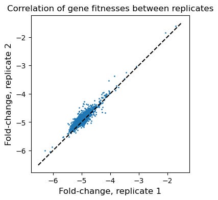
Overall, examining fitness at the gene level by aggregating across individual barcodes dramatically increases reproducibility.
Initial learnings
⏳ Early timepoints resolve moderate-fitness hits; late timepoints resolve mega-fitness hits
Selection is a complex, dynamic process, and our measured fitnesses are time-dependent due to stochasticity and clonal interference. At early timepoints, fitness effects begin to emerge but are weak due to less selection having taken place. At late timepoints, fitness effects are very apparent. Single barcodes begin to dominate the sample, and stochasticity is introduced since many species begin to die out due to clonal interference.
One core strength of this bioinformatics approach is the ability to construct distributions and conduct statistical tests. This lets us resolve statistically significant hits at early timepoints, pre-fixation. We actually observe more significant hits at earlier timepoints because no single/few fragments dominate the pool yet. Without sequencing, these would be very hard to detect.
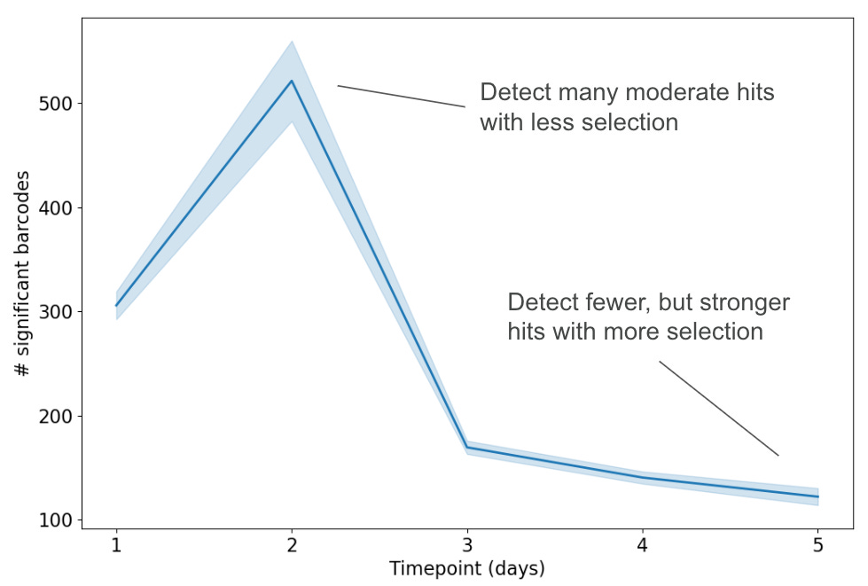
We can resolve statistically significant hits at early timepoints, pre-fixation.
Below is a plot of the number of barcodes with statistically significant high fitnesses over time. We see that there are more statistically significant barcodes at early timepoints. This is because, even though the super-high fitness winners emerge at late timepoints, this is at the cost of losing resolution of the less-high but still-significant fitness winners dying out. Because we sequence each timepoint, we can actually resolve these “medium” winners at early timepoints. Otherwise, if we only relied on experimental isolation of winners at the last timepoint, these medium hits would be virtually impossible to detect.
🗺️ We can map the fitness across the WHOLE donor genome!
Because of our long read data, we can map fragments back to the genome and generate fitness maps at genome scale with high resolution, unlocking the ability to query genes/operons of unknown function that can contribute to fitness advantages.
Below is a preliminary demonstration of this capacity. For each position in the reference H. elongata genome, we average the fitness (i.e. frequency fold-change value) of all barcode fragments that contain that position. From this we can generate a “peaks” map, along with a significance threshold based on a sampled null distribution constructed from the empty barcodes. Even by Day 1 we see some strong peaks emerge, such as galE, the strong winner from the above single-barcode trajectory analysis. opuE, the intermediate winner, displays a relatively weaker peak on this plot. Several other peaks are annotated with gene IDs and are candidates for further follow-up.
We can map fragments back to the genome and generate fitness maps at genome scale with high resolution.
Most importantly, this visualization aggregates across barcodes to the genome level, providing cleaner and much more resolved information about fitness contributions from the H. elongata genome compared to noisy single-barcode analysis. This type of data transformation yields a more biologically grounded plot to inform follow up investigations of hits!

What’s next?
So, where do we stand? We have a bioinformatics platform that vastly upgrades our engineering crank to produce quantitative readouts of evolutionary fitness contributions of inserted extremophile DNA sequences at scale. Our initial characterizations indicate that these measurements are reproducible within an experiment, at the per-barcode and per-gene level.
There are a few important directions we can go from here, which we’ll describe in an upcoming Bioinformatics Part 2 post:
Can we trust these numbers in a wider setting? While we are getting quantitative numbers for each library member, we need to investigate the reproducibility across different libraries, as well as reproducibility across experimental paradigms. Furthermore, do these fitness measurements translate to practical takeaways such as improved growth in a non-competitive assay?
Can we extend our experimental regimes? This proof of concept was conducted for a single extremophile genome inserted into a single host strain under a single selection condition. Can we scale up our experimental and computational facilities to multiplex along each of these three axes, including other Mars-relevant environmental conditions?
Can we investigate applications of AI/ML? Our dataset generation has the potential to enter the big data regime, at which point we could consider using modeling techniques to try to predict fitness effects from underlying DNA sequences. How will we know if these efforts will bear fruit?
How do we follow up on hits? Our bioinformatics data give a nuanced lens into the genes and/or operons that confer fitness advantage. How can we dissect our results for basic science (i.e. can we investigate genes of unknown function?) as well as for engineering applications (i.e. can we determine the best sequence for strain engineering?).
Zooming out, we need quantitative data at this scale to achieve our goals of making a Mars-ready biomanufacturing microbe. The engineering problem is vast across multiple scales. Here we built a library from a single extremophile (H. elongata), selected under a single condition (salt tolerance), and inserted into a single chassis microbe (E. coli). In principle, we could source gDNA from the entire tree of life. Furthermore, Mars possesses a multitude of harsh conditions besides high salt that we’ll need to evolve organisms to tolerate. Finally, there are many putative chassis organisms we could consider using in addition to E. coli.
To explore all of these unknowns, we’ll need to build up our experimental and computational capacities to deliver quantitative and actionable results to inform future evolution experiments.
Right now, the next step is to start turning the crank and scaling up our data generation efforts. If you’re interested to read Part II, or to follow our technical updates in general, please subscribe!
Work with us!
As these efforts continue, we would love to engage more with computational researchers. If you might be interested in this sort of genotype → phenotype data, please reach out and connect! We also welcome comments on these posts!
We are also growing the team to support these larger efforts. We will begin a search for two roles — a new member of the computational team, and an automation engineer — over the summer. If you want to stay updated, please fill out this form.
Cite as: Pioneer Labs Reports (2025). Laying the groundwork for data-driven evolution. figshare. https://doi.org/10.6084/m9.figshare.28970489.v1
 | A guest post by
|
I sincerely appreciate the openness. Providing the methods, data, interpretations, and next steps is a great way to lean into scientific communication! Thanks for the post
This is a very nice write-up! Thanks for sharing your work. I have a few questions:
1) When cloning the DNA+barcode into the E.Coli strains, is it always placed in the same location?
2) You show good correlation between replicates across your time course, I was wondering if any genes showed positive correlation across time points. Particularly your high fitness effect barcodes at day 5.
3) You averaged your fitness per position, but I wonder if you analyzed data after collating positions/inserts by operons you would have more consistent results. Particularly when using two very different microbes where you may miss interesting things if the full operon isn't included in the DNA insert (thus making any one part non-functional)